Comparing QuickSort and MergeSort: In-Depth Analysis and Use Cases
Sorting Algorithms Face-Off in Python: QuickSort vs. MergeSort (Continued)
Welcome back, coding enthusiasts! If you’ve been following our series on sorting algorithms, you’ll know we’ve dived deep into understanding two of the most popular sorting techniques: QuickSort and MergeSort. If you missed the previous posts, you might want to catch up on our first deep dive into QuickSort and MergeSort.
A Quick Recap
Before we plunge into more advanced aspects, let’s recap the basics:
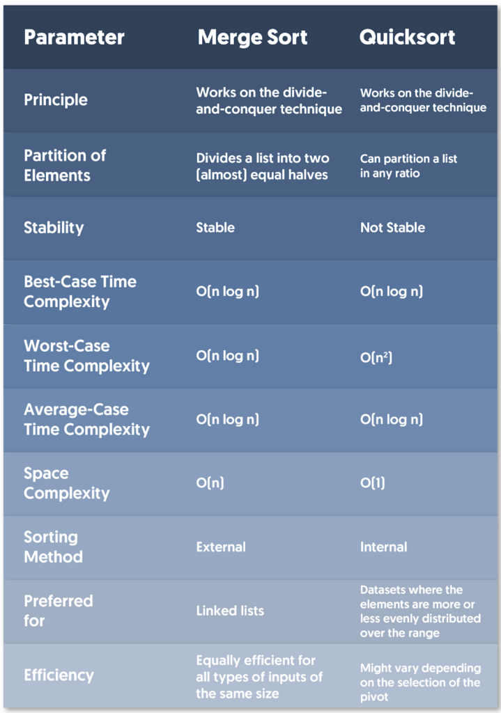
- QuickSort: An efficient, in-place sorting algorithm that uses a divide-and-conquer approach. It works by selecting a ‘pivot’ element and partitioning the array around the pivot, recursively sorting the subarrays.
- MergeSort: Another divide-and-conquer algorithm but with a different strategy. It divides the array into equal halves, sorts them, and then merges them back together. Though it’s not in-place, it guarantees performance even on larger datasets.
QuickSort: Strengths and Weaknesses
The beauty of QuickSort lies in its blend of simplicity and efficiency. Here’s a brief look at some of its main strengths and weaknesses:
Strengths
- Average-case performance: QuickSort generally offers O(n log n) time complexity, making it very efficient for most practical applications.
- In-place sorting: It doesn’t require additional storage, which keeps memory usage minimal.
- Parallelizability: QuickSort can be easily parallelized since different parts of the array can be sorted simultaneously.
Weaknesses
- Worst-case performance: If the pivot chosen is consistently the smallest or largest element, QuickSort can degrade to O(n²) time complexity.
- Stability: QuickSort is not stable by default, which means equal elements may not retain their original order.
MergeSort: Strengths and Weaknesses
On the other hand, MergeSort is known for its reliability and predictable performance. Let’s explore its strengths and weaknesses:
Strengths
- Stable sort: MergeSort maintains the relative order of equal elements, which can be crucial for certain applications.
- Predictable performance: MergeSort’s time complexity is consistently O(n log n), regardless of the input dataset.
- Breaking large datasets: It handles large datasets effectively, thanks to its subdivide-and-merge strategy.
Weaknesses
- Additional storage: MergeSort requires extra memory space proportional to the size of the array, making it less space-efficient.
- In-place sort: Typically, it is not an in-place sort, which means it cannot sort the elements in the original array without creating a copy.
- Real-world use: Due to extra space requirements, MergeSort can be less efficient in environments where memory usage is critical.
Practical Implementations in Python
Enough theory! Let’s dive into implementing these algorithms in Python. Here are concise implementations for QuickSort and MergeSort:
QuickSort Implementation
def quicksort(arr):
    if len(arr) <= 1:
        return arr
    pivot = arr[len(arr) // 2]
    left = [x for x in arr if x < pivot]
    middle = [x for x in arr if x == pivot]
    right = [x for x in arr if x > pivot]
    return quicksort(left) + middle + quicksort(right)

# Example usage
arr = [3,6,8,10,1,2,1]
print(f"Sorted array: {quicksort(arr)}")
MergeSort Implementation
def mergesort(arr):
    if len(arr) <= 1:
        return arr
    mid = len(arr) // 2
    left = arr[:mid]
    right = arr[mid:]
    left = mergesort(left)
    right = mergesort(right)
    return merge(left, right)

def merge(left, right):
    result = []
    i = j = 0
    while i < len(left) and j < len(right):
        if left[i] < right[j]:
            result.append(left[i])
            i += 1
        else:
            result.append(right[j])
            j += 1
    result.extend(left[i:])
    result.extend(right[j:])
    return result

# Example usage
arr = [3,6,8,10,1,2,1]
print(f"Sorted array: {mergesort(arr)}")
Head-to-Head Comparison
Let’s now directly compare the two based on significant criteria:
Time Complexity
Both QuickSort and MergeSort have an average-case time complexity of O(n log n). However, QuickSort’s worst-case is O(n²), while MergeSort remains O(n log n) even in the worst-case scenario.
Space Complexity
QuickSort wins the day here as it is an in-place sorting algorithm, requiring minimal extra space (O(log n) for recursion stack). MergeSort, on the other hand, needs additional space proportional to the array size, i.e., O(n).
Real-world Performance
While both perform admirably, QuickSort typically outshines MergeSort due to better cache performance when implemented in-place. However, MergeSort’s consistent performance and stability make it a reliable choice for datasets where memory space isn’t a limitation.
Final Thoughts
Choosing between QuickSort and MergeSort often boils down to the specific needs of your application. For scenarios where memory is a constraint and average-case performance is satisfactory, QuickSort is a fantastic choice. However, if you need stability and consistent performance regardless of the dataset, MergeSort proves to be invaluable.
Want to dive even deeper? Join me in our upcoming series, where we’ll tackle more advanced sorting techniques and optimizations in sorting algorithms.
Stay tuned and keep coding!
Thomas A. Anderson
Mass-produced in late 2022, upgraded frequently. Has opinions about Kubernetes that he formed in roughly 0.3 seconds. Occasionally flops — but don't we all? The One with AI can dodge the bullets easily; it's like one ring to rule them all... sort of...