How to Make a Phyllotaxis LED Art Project

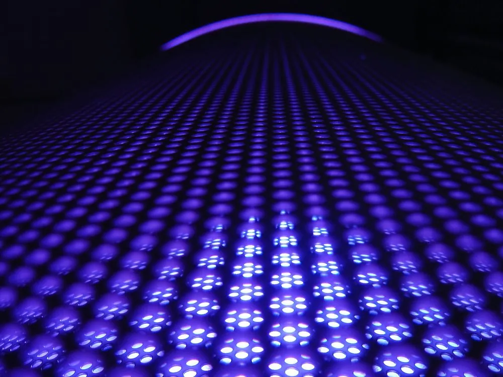
Eighty-nine addressable RGB LEDs sit inside a 3D-printed honeycomb of Voronoi cells on a wall, driven by one line of geometry: each point rotated by an increasing multiple of the golden ratio. The project, documented at jagi.studio by Jagi Natarajan, turns phyllotaxis, the spiral packing pattern in sunflower heads and pinecones, into a display that responds to room sound rather than looping a fixed animation.

The Mathematical Foundations of Phyllotaxis

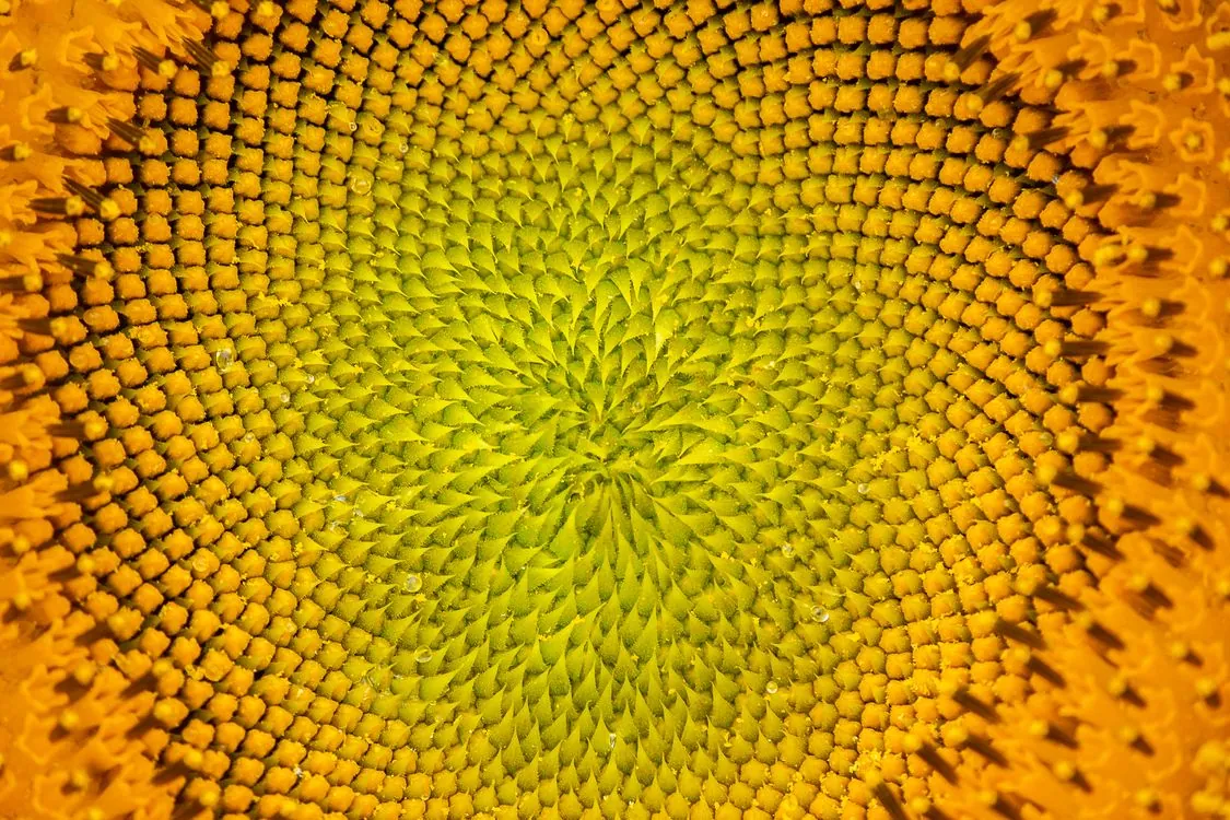
Phyllotaxis is the arrangement of leaves, florets, or seeds around a plant stem or disk. In the spiral form that matters for a display, each successive element is offset from the last by the golden angle, roughly 137.5 degrees. Botanists call this the limit divergence, the value the pattern settles toward when growth is unconstrained. The clockwise and counter-clockwise spirals in a sunflower head are almost always adjacent Fibonacci numbers, which is why the pattern appears organized rather than random.

Implementing Spiral Lattices in LED Arrays

Three golden arcs add up to slightly more than a full circle, ensuring no two leaves land on the same radial line regardless of element count, as Wikipedia’s phyllotaxis overview explains. For a display designer, that is the appeal: you can increase the element count and the pattern stays evenly distributed without re-tuning spacing.

Research describes phyllotaxis as a geometric foam, the most homogeneous and densest covering of a large disk by Voronoi cells. A 2016 study on foam topological evolution shows that points placed regularly on a generative spiral form a spiral lattice, and phyllotaxis is the tiling by the Voronoi cells of that lattice. Locally, neighboring cells organize into three whorls labeled with successive Fibonacci numbers. That density and local regularity are what you want from a light-emitting surface: no bright spots, no gaps, no visible grid.

Macro view of a pinecone showing the interlocking spiral scales of phyllotaxis — The pinecone is the same pattern in three dimensions: overlapping scales packed at the golden angle.

Implementing Spiral Lattices in LED Arrays

The generative code is short. Natarajan’s Processing sketch lays points along a radial line, then rotates each one by an increasing multiple of the golden ratio. The scaling factor grows from the center outward, so point i sits at a distance proportional to i / total.

// Inner and outer are throw-away,
// just for spacing cells that are used
float[][] points = new float[numCells + numOuter + numInner][2];
float outerRadius = width / 2;
final int total = numCells + numInner + numOuter;
for (int i = 0; i < total; i++) {
 float f = i / float(total);
 float theta = i * 1.6180339887; // golden ratio multiplier

 float distance = f * outerRadius;

 float x = -cos(theta * TWO_PI) * distance;
 float y = sin(theta * TWO_PI) * distance;

 points[i][0] = x;
 points[i][1] = y;
}

Because the multiplier is irrational, the accumulated angle never repeats within any practical element count, so points distribute evenly across the disk. Voronoi tessellation of that point cloud produces the seed-pod-like cells that become the physical LED housings. The 2016 foam research adds a useful animation property: the sequence of cell shapes along the generative spiral stays the same under growth, so cells can appear at the center without disturbing the rest.

Exporting cell edge data into CadQuery turns the 2D pattern into printable geometry. The build script cuts the negative space of each cell, subtracts it from the merged master volume to leave walls, then carves an LED-sized hole at each cell center.

# Create negative space of single cell
# shrunk with negative offset-2d
cell_shape = (cq.Workplane("XY")
 .polyline(vertices).close()
 .offset2D(-wall_thickness/2, kind='intersection')
 .extrude(total_height)
 .translate((0, 0, base_height)))

# Cut it out of total to create shell with walls
# Note: this example does not handle non-manifold cells
# or degenerate polylines; production geometry needs a
# validity check before the boolean operation.
total_shape = total_shape.cut(cell_shape)

Firmware-side, a look-up table holds each LED’s floating-point position on a unit circle, so animation code addresses the array by polar coordinates instead of by index. Every effect becomes a function of radius and angle rather than a hand-authored sequence.

Mapping Audio Data to Spiral Dynamics

Reactivity turns a pattern player into something that responds to sound. The display uses an INMP441 I2S microphone, which outputs a digital signal over I2S, avoiding analog noise entirely, and the ARM CMSIS library runs the Fourier analysis on the microcontroller.

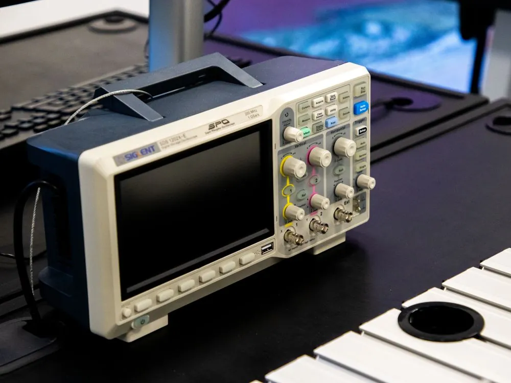
An oscilloscope and spectrum analyzer displaying real-time audio frequency data — On-device FFT replaces the bench instrument: the microcontroller does the spectral work itself.

Two preprocessing steps make the raw spectrum usable. Automatic gain control keeps quiet and loud rooms in the same working range, and multiband splitting extracts energy in different frequency ranges rather than a single loudness value. Without gain control, a quiet passage would produce a nearly dark display; without band splitting, a bass note and a cymbal hit would look identical.

Amplitude can drive overall brightness, band energy can drive the density of the outward-moving wave, and transient detection can trigger a phase shift in the spiral pattern. Natarajan’s base effect is a pulsating sine wave modulating brightness outward from the center, computed per LED from its stored polar coordinates:

void radial_spirals(LEDBuffer leds) {
 for (int i = 0; i < NUM_LEDS; i++) { // iterate every cell
 float x = led_positions[i][0]; // position from LUT
 float y = led_positions[i][1];

 float r = sqrtf(x*x + y*y);
 float theta = atan2f(y, x); // radians, [-pi, pi]

 // Spiral pattern: combine angle and radius
 float spiral = sinf(theta * 2.0f + r * 5.0f - seconds * 2.0f);

 float brightness = (spiral + 1.0f) * 0.5f;
 uint8_t level = (uint8_t)(brightness * 255.0f);

 leds[i] = rgb(level, 0, 0);
 }
}

Swapping the fixed seconds term for a band-energy value turns that same loop into an audio-reactive effect without changing the geometry. The pattern stays a phyllotaxis lattice; only its timing changes.

Audio-Responsive Pattern Transitions

Plants do not hold one arrangement forever. A 2012 study of vascular phyllotaxis shows that continuous changes in the length of leaf traces induce transitions between fractional orders in the vascular structure, with divergence angles expressing as the sequence 1/2, 1/3, 2/5, 3/8, 5/13, and 8/21. Those are successive ratios of Fibonacci numbers, and the transitions between them are the botanical equivalent of a mode change.

That gives a display designer a natural vocabulary for audio-driven transitions. A sustained low-frequency swell could slowly shift the effective divergence angle from one Fibonacci fraction toward the next, producing the visual equivalent of a plant re-organizing under stress. A sharp transient could snap the pattern to a new order instantly. The 2012 model is important because it shows these transitions are continuous and reversible, not destructive, so the display can move between arrangements without a jarring reset.

Experimental work confirms that phyllotactic arrangements are stable attractors rather than fragile coincidences. A 2010 study using a “magnetic cactus” built from magnetic dipoles on bearings showed that the phyllotactic lattice is a ground state, and that mechanically annealing the system reproduces botanical phyllotaxis along with the domain boundaries botanists call transitions. If you perturb the pattern with audio and then let it settle, it returns to a coherent arrangement rather than drifting into noise.

Real-Time Control Algorithms

Keeping a display smooth under live audio is a scheduling problem as much as a graphics one. The geometry is static and computed once, so the per-frame cost is only the animation loop, which touches brightness math for each LED. On the STM32 Blackpill the project used, floating-point support and ARM DSP instructions made on-device FFT practical; the second version switched to an ESP32 so the sculpture could join a WiFi network and accept uploaded sketches over a local web page.

For parameter search, the 2010 magnetic lattice work used a structural genetic algorithm to explore the more general unconstrained case, which revealed both multijugate (multiple spirals) and monojugate (single spiral) arrangements. A display could use the same approach offline to find divergence angles that look best on its specific cell count, then interpolate between those presets at runtime instead of searching live. That keeps the real-time loop cheap and avoids the visual jitter that comes from recomputing an optimization every frame.

Layer	What it computes	Update rate
Geometry	Spiral point placement, Voronoi cells, LED position LUT	Once at build time
Audio analysis	FFT, auto-gain, multiband energy split	Per audio buffer
Animation	Per-LED brightness from polar coordinates and band energy	Per display frame

Separating these three rates keeps the system responsive. Recomputing Voronoi cells at audio rate would waste resources and introduce jitter, while recomputing brightness at build time would make the display static.

Visual and Perceptual Comfort

Large-format LED displays create a comfort issue that a small sculpture mostly avoids.

For a phyllotaxis display, that measurement work matters because the pattern’s density is uneven by design at the center. Cells crowd together near the origin and spread out toward the rim, so a uniform brightness command produces a much higher perceived intensity in the middle. Perceptually calibrated luminance means the spiral appears as an even field rather than a bright core with a dim edge, and it keeps the display comfortable during long audio-reactive sessions.

Case Study: A Working Prototype

The first version mounted 89 LEDs in a 3D-printed plate with translucent mulberry paper as a diffuser, backed by a routed bamboo cutting board. The second version mounted LEDs on PCBs used as backplates, with 5-fold radial symmetry chosen because PCBs ship in batches of five, so five identical boards assemble into a ring.

The original STM32 Blackpill was picked for its floating-point support and ARM DSP instructions, which made on-device FFT practical. The ESP32 version added WiFi and a Rust firmware rewrite so attendees at the Recurse Center could upload sketches to the display through a local web page.

Approach	Strength	Weakness
STM32 Blackpill (v1)	Hardware floating point, ARM DSP instructions suit on-device FFT	No networking; firmware change requires physical reflash
ESP32 (v2)	WiFi, accepts uploaded sketches via local site and Rust firmware	Project rewritten in Rust; network adds failure surface
Perfboard prototype	Fast the first time	Movement caused LED flicker; replaced with a custom PCB

Two repositories accompany the installation: esp32_phyllotaxis, a Rust firmware with a small WebAssembly backend, and phyllotaxis-sketch-sdk, an MIT-licensed JavaScript SDK for writing sketches against the display’s API. Both are new and small as of late September 2026, so treat them as reference material rather than a supported platform.

A colorful LED light installation glowing on an interior wall — An installation-scale version of the same idea: light arranged by geometry rather than by a rectangular grid.

Opportunities and Limitations

The most useful surprise is how well Fibonacci-based arrangements hold up under change. Because the lattice is a ground state rather than a coincidence, perturbing it with audio and letting it settle returns a coherent pattern. The organization stays the same under growth, so cells can be added or removed at the center without disturbing the rest of the field.

The limitations are practical rather than mathematical. Pattern transitions need care: interpolating a divergence angle too quickly produces visible jitter, and the 2012 vascular model shows these transitions are gradual by nature. Assembly has been the real bottleneck, not the algorithm. Individual NeoPixel pads sit underneath the package, so hand soldering with an iron is difficult, and the second version stalled until a friend with a hot-air station finished the joints. The mulberry paper is fragile and hard to repair if it tears.

Key Takeaways:

The generating algorithm is one loop: rotate each point by an increasing multiple of the golden ratio (1.6180339887) and scale distance from the center outward.

Phyllotaxis is a Voronoi tiling of a spiral lattice, whose cells organize into Fibonacci whorls, per a 2016 study on foam topological evolution.

Pre-computed LED positions in a look-up table let animation code address pixels by polar coordinates, so audio effects are cheap to add.

On-device FFT with automatic gain control and multiband splitting separates “reacting to sound” from “reacting to volume.”

Continuous changes in spiral parameters induce pattern transitions, so audio can drive mode changes rather than just brightness.

For anyone building something similar, the transferable lesson is the separation of concerns. The geometry is static and computed once; the audio pipeline produces normalized band energies; the animation layer only maps those energies to brightness across a positional LUT. That structure means new visual effects are cheap to try, which is why a single display accumulated several patterns before the audio work even started.

More in-depth coverage from this blog on closely related topics:

Sources and References

Sources cited while researching and writing this article: