AI Data Center Emissions by Region

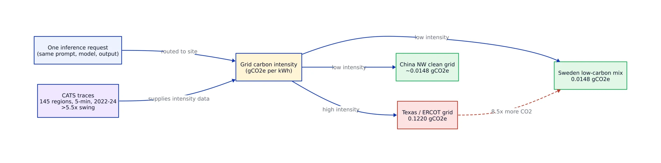
Send one inference request to the service sitting next to the user and it emits 0.1220 gCO2e. Send the identical request to a clean-electricity site on China’s northwest grid and the estimate falls to 0.0148 gCO2e. Same prompt, same model, same output, an 88% difference in carbon, and that pair of numbers is the buyer case in GreenPassport Carbon Accounting (GPCA), a September 2026 paper on request-level carbon accounting.

Where a Request Runs, and When

Inference crosses regional boundaries as a matter of course. A prompt travels to a remote data center, GPUs convert it into tokens, and the tokens return over a network path with its own energy cost. Serving hardware, electricity mix, and route all differ by site, so a regional average describes none of the requests that actually ran. The CATS authors gave the gap between where capacity sits and where clean power is cheapest a name: the siting-carbon mismatch.

Cooling and Capacity as the Second Constraint

What Request-Level Accounting Requires

Attribution is where carbon dashboards fall apart. GPCA defines a boundary that has to hold across every request it reports: the service, the serving site, the route, a local comparator, an uncertainty figure, and data provenance. The system estimates serving carbon and route carbon as separate terms, then picks a reporting level from however much documentation actually exists for that request.

Against six accounting baselines and four energy-prediction baselines, GPCA reduced median absolute percentage error by 56.3% and median absolute error by 15.5% relative to EcoLogits, under an aligned accelerator-energy boundary. It also produced zero rule overstatement in deterministic conformance tests. Overstating a saving is worse than reporting none, because an inflated figure cannot be audited back to a meter.

Method	Measured result	Test conditions
Spatial shifting (CATS)	38.4% CO2 reduction vs speed-first baseline	24-hour trace, 600,000 tasks, fleet use of 0.37
Temporal shifting (CATS)	16% CO2 savings, SLA violations at 3.27%	Same 24-hour trace, bounded SLA
GPCA request accounting	56.3% lower median absolute percentage error, 15.5% lower median absolute error	vs EcoLogits, aligned accelerator-energy boundary
Route selection, CN-West	0.0148 vs 0.1220 gCO2e per request, 88% lower	GPCA buyer case, clean-electricity scenario
Thermal AI surrogate	10,000x speedup over high-fidelity CFD	Unseen data center designs, millisecond temperature prediction

The buyer case shows how completely route choice can dominate. Two orders of magnitude separate the best and worst paths for identical work, and no amount of accelerator tuning closes that gap. The limitation is documentation. A reporting level can only be as precise as the data behind it, and most providers publish neither per-request energy nor network route emissions, so a large share of requests fall back to a coarser estimate than the paper’s headline error rate implies.

The Metric Problem: Marginal Carbon Intensity

Most carbon-aware schedulers optimize against marginal carbon intensity (MCI), the estimated emissions change from adding one more unit of load. A 2025 statement paper, Moving Beyond Marginal Carbon Intensity, argues the metric is neither reliable nor actionable for accounting or for grid flexibility. The listed failures are concrete: MCI is not directly observable, it leans on opaque predictive models, and it has no verifiability. It does not reflect curtailment caused by high-carbon sources, and it says nothing about how much excess power is actually on the wire.

The proposed replacements are narrower and harder to game. Report excess power directly instead of inferring it. Model storage and grid stability explicitly. Tie the signal to granular renewable energy certificate markets. Each substitute converts the engineering task from forecasting a derived number into measuring a physical quantity, which is a different data pipeline with different failure modes.

For a team shipping a scheduler now, MCI remains a proxy and should be labeled as one. If a dashboard claims a 30% reduction on forecast marginal intensity, that figure carries forecast error the dashboard does not show. Where a direct measurement of curtailed power exists, it is the better input to a routing decision.

Scheduling: Spatial vs Temporal Shifting

The carbon cost of a placement is energy consumed multiplied by grid intensity at that moment. Both terms are variable and both are usually estimated from a handful of inputs: accelerator type, wall-clock duration, facility overhead multiplier, grid mix. A minimal implementation makes the latency-versus-emissions trade explicit, which is the part commercial schedulers hide.

# Minimal carbon-aware placement sketch.
# Note: production use needs live grid-intensity feeds, per-GPU power curves,
# route (network) emissions, queueing and SLA-aware admission control.
# Intensity and wattage values below are illustrative placeholders, not measurements.

REGIONS = {"us-east": 410.0, "us-west": 190.0, "eu-north": 45.0} # gCO2e/kWh
GPU_WATTS = {"h100": 700.0, "l40s": 350.0} # illustrative TDP-style values
PUE = 1.2 # facility overhead multiplier

def request_grams(gpu: str, region: str, seconds: float) -> float:
 kwh = GPU_WATTS[gpu] * seconds / 3_600_000 * PUE
 return kwh * REGIONS[region]

def pick_region(gpu: str, seconds: float, latency_budget_ms: int,
 region_latency_ms: dict) -> str:
 eligible = [r for r in REGIONS if region_latency_ms[r] <= latency_budget_ms]
 if not eligible:
 raise ValueError("no region inside latency budget")
 return min(eligible, key=lambda r: request_grams(gpu, r, seconds))

print(pick_region("h100", 2.5, 120, {"us-east": 40, "us-west": 70, "eu-north": 190}))
# expected: us-west, since eu-north misses the 120 ms budget

The latency filter is what separates a realistic scheduler from a carbon-only optimizer. In the CATS trace, temporal shifting could defer work but had to stay inside an SLA, and it still produced 3.27% violations. Spatial shifting won the larger reduction for a structural reason: regional intensity differences exceed diurnal ones in most grids. It also adds network emissions that a naive model omits entirely, which is why GPCA estimates serving and route carbon as separate terms instead of folding them into one multiplier.

Cooling and Capacity as the Second Constraint

Moving work changes more than the emissions ledger. LLM workloads create localized hotspots, and the thermal spikes from training and inference bursts make cooling response hard to predict, so capacity planning normally leans on high-fidelity CFD simulation that is expensive for every design. An October 2026 paper trains an AI surrogate on rack power, server power, server placement, and HVAC settings to predict temperature in milliseconds. Tested against CFD on unseen designs, the model reports a 10,000x speedup.

The surrogate drives a planning framework that optimizes workload distribution and cooling efficiency together. That coupling matters here. A region that looks clean on paper but is thermally constrained will throttle, stretching job duration and eating the intensity advantage it was chosen for. Any scheduler blind to facility headroom hands its savings back as longer runtimes.

Reporting Carbon at the Benchmark Level

Model selection is still mostly a single-objective decision on accuracy, BLEU, or mAP, with energy and emissions absent from the table. AI-CARE, proposed in a February 2026 paper, adds energy consumption and carbon reporting beside those metrics and introduces a carbon-performance tradeoff curve plotting the Pareto frontier between quality and carbon cost. The authors report that carbon-aware benchmarking changes the relative ranking of models, which makes an accuracy leaderboard a misleading guide to deployment cost.

The tool is published at github.com/USD-AI-ResearchLab/ai-care. Its value hinges on the same boundary problem GPCA attacks: a carbon number with no stated accelerator-energy boundary, grid region, and measurement window cannot be compared across papers. Run the same model in a low-carbon region and it will beat its own score from a coal-heavy one, with zero change to the architecture.

Where These Methods Break

Forecast error flows straight into the claimed saving. Temporal shifting depends on day-ahead intensity forecasts, and the MCI critique applies just as forcefully to any derived signal with no observation behind it. Spatial shifting assumes you know per-request energy by accelerator type, and most providers publish nothing of the sort, leaving teams to infer from thermal design power and use.

use changes the arithmetic. The 38.4% figure holds at fleet use of 0.37 on a 600,000-task trace, where a large share of capacity is idle and relocating work costs little. Push use high and the slack disappears, so a placement decision starts trading against queue delay. Run the fleet near idle and there is slack everywhere but most of the hardware is wasted. Scale matters too: deferring millions of small requests is cheap, while deferring a training run that holds thousands of GPUs for weeks is a contract negotiation wearing a scheduler's clothes.

The defensible 2026 position is that carbon-aware inference is measurable and worth doing at the request level, but the numbers move with the boundary drawn around them. Declare the boundary, publish the trace, and treat marginal-intensity savings as estimates rather than measurements. Teams that do this find the 38.4% and 16% figures reproducible in direction, if not in magnitude.

More in-depth coverage from this blog on closely related topics:

Sources and References

Sources cited while researching and writing this article: