Fast Integer Multiplication Algorithm

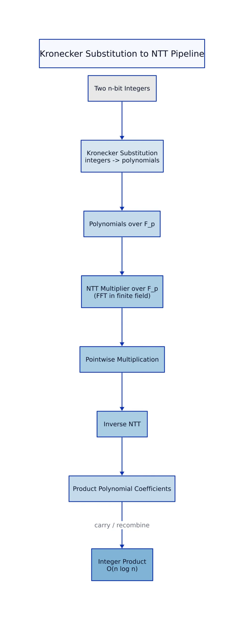
In March 2019, David Harvey and Joris van der Hoeven posted a proof that two n-bit integers can be multiplied in O(n log n) bit operations. Schönhage and Strassen had introduced FFT-based multiplication in 1971 and conjectured that O(n log n) was the floor; closing that 48-year gap made the rounds on every algorithms blog. It will not speed up a single line of the big-integer code you ship.

The Bound and the Ladder It Topped

The announcement coverage was straightforward: Math Scholar’s write-up and Richard Lipton’s post both framed the result as the end of a decades-long chase. What matters technically is the shape of the ladder that preceded it, because that shape explains why the final rung is worth so little at practical sizes.

The prior record was not one number but a family: O(n log n K^{log* n}). The iterated logarithm log* n counts how many times you apply log before the value drops below 1, and it grows so slowly that it behaves like a small constant. For a 2⁶⁵⁵³⁶-bit integer, log* n is 5. So the jump from 4^{log* n} to 1 is at most a factor of 4⁵ = 1,024, and the constant hidden inside the O(n log n) proof eats into even that. The theorem is real and the improvement is real; the crossover point where FFT-based multiplication starts beating grade-school loops did not move.

Two intermediate steps matter for anyone reading the papers. The 2018 lattice-vector paper proved O(n log n 4^{log* n}) unconditionally, leaning “in an essential way on Minkowski’s theorem concerning lattice vectors in symmetric convex sets” rather than on unproved number-theoretic hypotheses. The earlier explicit-bound work gave O(n log n K^{log* n}) with K = 8, noting that an optimised variant of Fürer’s algorithm reaches only K = 16, a factor of 2^{log* n} worse.

Measuring Big-Integer Scaling on Your Own Hardware

Before trusting any asymptotic claim, measure the routine you already call. This script doubles the operand width five times and prints the growth ratio between consecutive sizes; on a Karatsuba-class implementation the ratio lands near 3x per doubling, well above the 2x that a truly linear algorithm would show.

import time

def bench(bits: int, trials: int = 5) -> float:
    a = (1 << bits) - 1  # all bits set
    b = (1 << bits) - 0x9E3  # uneven operand, closer to real key material
    best = float("inf")
    for _ in range(trials):
        t0 = time.perf_counter()
        c = a * b
        best = min(best, time.perf_counter() - t0)
    assert c > 0
    assert c.bit_length() in (2 * bits - 1, 2 * bits)
    return best

prev = None
for bits in (1 << 14, 1 << 15, 1 << 16, 1 << 17, 1 << 18):
    t = bench(bits)
    ratio = f"{t / prev:5.2f}x" if prev else " - "
    print(f"{bits:>7} bits {t * 1e3:7.3f} ms {ratio}")
    prev = t

# Illustrative run (x86-64 container, CPython 3.12.15; absolute times vary):
# 16384 bits 0.222 ms -
# 32768 bits 0.677 ms 3.05x
# 65536 bits 2.088 ms 3.08x
# 131072 bits 6.433 ms 3.08x
# 262144 bits 19.714 ms 3.06x
#
# Note: a production benchmark should pin the CPU, disable frequency scaling,
# and repeat across separate processes; this measures one multiply per trial.

The ratios are noisy, but they cluster around 3x, roughly 2^1.6, which is what the sub-quadratic tier of algorithms that mainstream runtimes ship predicts. Nothing in the 2019 proof changes that slope, because no mainstream runtime implements the new algorithm. If your workload multiplies multi-megabit integers, the constants you can tune today live in library selection and in how many times you copy the operands, not in the exponent.

Kronecker Substitution: Integers Into Polynomials

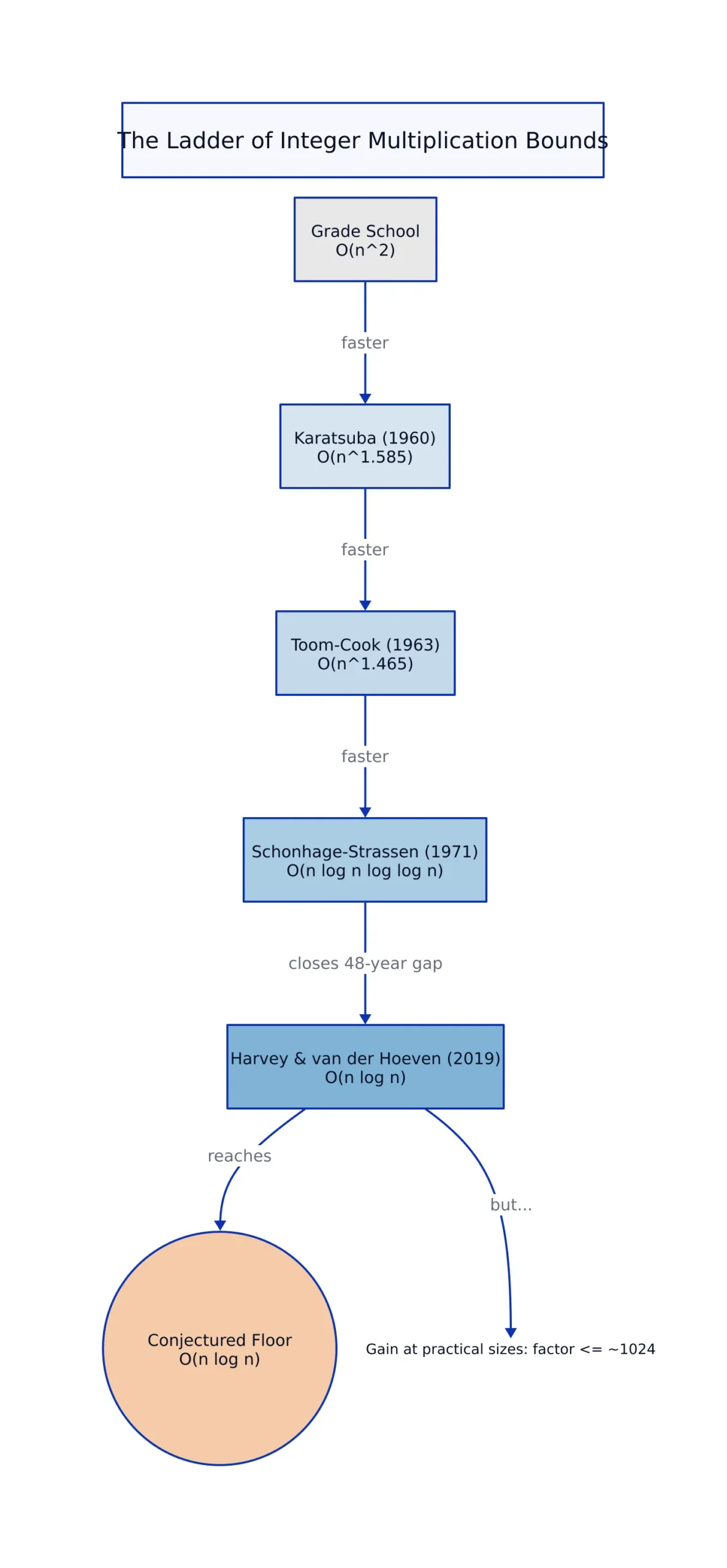
The standard reduction behind many fast integer multipliers is Kronecker substitution: chop each integer into fixed-width limbs, treat the limb array as polynomial coefficients, multiply the polynomials, then repack. Each output coefficient is a sum of up to min(len(a), len(b)) products of limb-sized values. There are two safe ways to repack. Carry-normalize the coefficients back into the original 2³² base, as the code below does, or pack each coefficient at a wider stride B. For the wide-stride variant, B must be wide enough to hold the largest coefficient: at least twice the limb width plus ceil(log2(min(len(a), len(b)))) bits, with a guard bit if the bound is exact. The common bug is mixing the two: split at 32 bits, then pack at 72 without carrying or unpacking at 72.

Note: The following code is an illustrative example and has not been verified against official documentation. Please refer to the official docs for production-ready code.

LIMB_BITS = 32

def to_limbs(n: int, width: int) -> list[int]:
    mask = (1 << width) - 1
    limbs = []
    while n:
        limbs.append(n & mask)
        n >>= width
    return limbs or [0]

def from_coeffs(coeffs: list[int], width: int) -> int:
    mask = (1 << width) - 1
    digits = []
    carry = 0
    for coeff in coeffs:
        total = coeff + carry
        digits.append(total & mask)
        carry = total >> width
    while carry:
        digits.append(carry & mask)
        carry >>= width
    out = 0
    for digit in reversed(digits):
        out = (out << width) | digit
    return out

def schoolbook(a: list[int], b: list[int]) -> list[int]:
    out = [0] * (len(a) + len(b) - 1)
    for i, ai in enumerate(a):
        for j, bj in enumerate(b):
            out[i + j] += ai * bj
    return out

a = 0xDEADBEEFCAFEBABE1234567890ABCDEF
b = 0xFEDCBA9876543210F0E1D2C3B4A59687

packed = from_coeffs(schoolbook(to_limbs(a, 32), to_limbs(b, 32)), LIMB_BITS)
print(packed == a * b) # True
print(hex(packed)[:10]) # 0xddb06310... (same prefix as hex(a * b))

# Note: production use should replace schoolbook with an NTT or FFT
# for large operands; from_coeffs carries in the same base as to_limbs.

The earlier version split at 32 bits but packed at 72, so it represented the product in base 2⁷² while the operands were base 2³²; the result was False. Setting LIMB_BITS to 60 only moves where the assertion fails. Either carry in base 2³², as above, or use one consistent wide stride with the coefficient bound. For large inputs, replace schoolbook with an NTT or FFT; the width and transform size become mandatory bookkeeping.

An NTT Multiplier Over F_p

Number-theoretic transforms dodge the precision problems of floating-point FFT by doing all arithmetic modulo a prime with a large power-of-two factor in p – 1. The modulus 998244353 is a common choice because p – 1 = 998244352 = 119 * 2²³, which supports transforms up to 8,388,608 points.

MOD = 998244353
ROOT = 3

def ntt(a: list[int], invert: bool) -> None:
    n = len(a)
    j = 0
    for i in range(1, n):
        bit = n >> 1
        while j & bit:
            j ^= bit
            bit >>= 1
        j |= bit
        if i < j:
            a[i], a[j] = a[j], a[i]
    length = 2
    while length <= n:
        wlen = pow(ROOT, (MOD - 1) // length, MOD)
        if invert:
            wlen = pow(wlen, MOD - 2, MOD)
        for start in range(0, n, length):
            w = 1
            half = length >> 1
            for k in range(start, start + half):
                u = a[k]
                v = a[k + half] * w % MOD
                a[k] = (u + v) % MOD
                a[k + half] = (u - v) % MOD
                w = w * wlen % MOD
        length <<= 1
    if invert:
        n_inv = pow(n, MOD - 2, MOD)
        for i in range(n):
            a[i] = a[i] * n_inv % MOD

def poly_mul_ntt(a: list[int], b: list[int]) -> list[int]:
    size = 1
    while size < len(a) + len(b) - 1:
        size <<= 1
    fa = a + [0] * (size - len(a))
    fb = b + [0] * (size - len(b))
    ntt(fa, False)
    ntt(fb, False)
    for i in range(size):
        fa[i] = fa[i] * fb[i] % MOD
    ntt(fa, True)
    return fa[:len(a) + len(b) - 1]

def naive(a, b):
    out = [0] * (len(a) + len(b) - 1)
    for i, ai in enumerate(a):
        for j, bj in enumerate(b):
            out[i + j] = (out[i + j] + ai * bj) % MOD
    return out

x = [123456789, 987654321, 555555555, 111111111]
y = [314159265, 271828182, 161803398]

print(poly_mul_ntt(x, y) == naive(x, y))  # True
print(len(poly_mul_ntt(x, y)))  # 6

# Note: production use should cap the transform size to the modulus's
# 2-adic headroom, reduce inputs mod p first, and reject oversized batches.

The last mile of the ladder is bookkeeping at the transition points. Van der Hoeven’s truncated Fourier transform was introduced to smooth the running-time jumps plain FFT shows at power-of-two input sizes, and in-place forward and inverse variants reach O(n log n) time with O(1) auxiliary space. If you have watched a transform-heavy job slow down when a batch crossed a power-of-two boundary, that is the effect those variants address. The same machinery is what makes polynomial multiplication over F_p cheap: Fürer-type bounds for F_p[X] give O(n log n 8^{log* n} log p), improving on the earlier O(n log n log log n log p).

The log-star Ladder in Numbers

Each row below is a published bound for multiplying two n-bit integers, in the order the field climbed them.

Bound	Year	Source	What changed
O(n log n K^{log* n}), K = 8	2014	arXiv:1407.3360	Explicit constant; the authors note Fürer’s optimised variant only reaches K = 16
O(n log n 6^{log* n})	2017	arXiv:1712.03693	Cited there as the previous best known bound
O(n log n (4√2)^{log* n})	2017	arXiv:1712.03693	Cyclotomic coefficient rings; base drops from 6 to about 5.66
O(n log n 4^{log* n}), unconditional	2018	arXiv:1802.07932	Drops all unproved number-theoretic hypotheses via Minkowski’s lattice theorem
O(n log n)	2019	Harvey and van der Hoeven (Annals 2021)	Iterated-logarithm factor removed entirely

Read down the last column and a pattern appears: most of the progress between 2014 and 2019 came from shrinking a constant, not from changing the shape of the curve. Only the bottom row removes the log* term completely, and its hidden constants are not small. That is why the practical ordering of these algorithms on a 4,096-bit modulus looks nothing like the table.

Choosing a Big-Integer Routine in Production

Practical multipliers are hybrids. Below some threshold a quadratic loop wins because it has no setup cost and fits in cache. In the middle range a divide-and-conquer split wins. Above that, transform-based methods take over. Any library you pick encodes cutoffs tuned to its own coefficient representation, so the useful comparison is measured throughput on your operand sizes, not the exponent printed in a paper.

Two trade-offs deserve attention. Floating-point FFT multipliers are fast but need precision guarantees: as transform length grows, coefficient magnitudes grow with it, and the round-off analysis has to be redone for the new size. Modular NTT multipliers avoid precision entirely but pay a modular-reduction cost per butterfly and are limited by the 2-adic headroom of the chosen prime. Operands that exceed that headroom force you into several primes plus a Chinese remainder reconstruction, or back to a different method for the largest sizes.

There is also an honest reason the 2019 result has not shown up in mainstream runtimes. A question on the Matter Modeling Stack Exchange asked directly whether the O(n log n) discovery had a practical outcome, and the way the question is phrased tells you what practitioners expected. The constants are large, the implementation surface is significant, and the realistic crossover sits far beyond the operand sizes most applications touch. For 2,048-bit or 4,096-bit modular arithmetic in TLS, the whole question is moot: those operands are small enough that a Karatsuba-class routine beats anything FFT-based.

Where it does matter is the fringe: exact integer arithmetic on multi-megabit operands, polynomial multiplication in computer algebra, and cryptographic parameter generation at large widths. If you work there, benchmark the shipped library first, then reach for a transform implementation. If you do not, the correct action in 2026 is to keep calling the built-in type, because the asymptotically best algorithm can be the slowest one for your data.

Sources: arXiv:1712.03693, arXiv:1802.07932, arXiv:1407.3360, arXiv:1407.3361, arXiv:1001.5272, Schönhage–Strassen algorithm on Wikipedia.

More in-depth coverage from this blog on closely related topics:

Sources and References

Sources cited while researching and writing this article: